Exploring Graph Algorithms : Dijkstra Algorithm

Today, we dive into the fascinating world of Graph algorithms and uncover their most captivating mysteries — Dijkstra Algorithm . Get ready to embark that will challenge your minds and you will come to know about the power of Graphs.

Introduction to Graph Algorithms

Graph algorithms are a powerful tool for solving a wide variety of problems . These are used to solve problems on graphs , such as finding the shortest path between two nodes , finding the maximum flow in a network or detecting communities in a social network.

Graph algorithms are used wide variety of applications such as

Transportation : for finding the shortest route between two points
Social Networks : detecting spam users , identifying influential users
Computer Science : compiling programs , optimizing network performance and malware detection

There are few basic types of algorithms such as “Breadth-first search(BFS)” , “depth-first search(DFS)”, Dijkstra algorithm ,Bellman-Ford algorithm etc. and also we have few advanced type of algorithms such as “Matching algorithm” , “Clustering algorithm”, and Maximum flow algorithm etc. It also works on both directed(edges are present for a graph) and undirected graph(there will be no edges for a graph) .

Graph algorithm can be implemented in different programming languages and software Libraries . Some popular graph libraries include

NetworkX : A python library for graph implementation and graph manipulation
GraphLab : A distributed graph computing framework
Neo4j : A graph database management system

One of the fundamental tasks in graph theory is Dijkstra Algorithm.

Overview of Dijkstra’s Algorithm

Dijkstra’s algorithm is a graph algorithm that finds you the shortest path between a single source node and all other nodes in a graph . It is a greedy algorithm , that it makes the locally optimal choice at each step in order to reach the globally optimal solution.

CODE:

import heapq

def dijkstra(graph, start): # Initialize distances and visited nodes distances = {node: float('infinity') for node in graph} distances[start] = 0 priority_queue = [(0, start)]

while priority_queue:
    current_distance, current_node = heapq.heappop(priority_queue)

    if current_distance > distances[current_node]:
        continue

    for neighbor, weight in graph[current_node].items():
        distance = current_distance + weight

        if distance < distances[neighbor]:
            distances[neighbor] = distance
            heapq.heappush(priority_queue, (distance, neighbor))

return distances

User-defined graph input

graph = { 'A': {'B': 1, 'C': 4}, 'B': {'A': 1, 'C': 2, 'D': 5}, 'C': {'A': 4, 'B': 2, 'D': 1}, 'D': {'B': 5, 'C': 1} }

start_node = input("Enter the starting node: ").upper()

Check if the starting node is in the graph

if start_node not in graph: print("Invalid starting node.") else: result = dijkstra(graph, start_node) print("Shortest distances from node {}:".format(start_node)) for node, distance in result.items(): print("To {}: {}".format(node, distance))

Code Explanation :

Initialize a set of visited nodes and a set of unvisited nodes . The visited set is initially empty, and the unvisited set contains all the nodes in the graph .
select the source node and add it into the visited set .
For each neighbor of the source node, calculate the shortest distance from the source node to the neighbor. If the calculated distance is shortest than the current distance sorted for the neighbor , update the neighbor’s distance and add it into the priority queue.
Once all nodes have been visited, the distance of each node is the shortest distance from the source node to that node
Here the algorithm terminates, when all of the nodes in the graph have been visited. At this point , the tentative distance of each node is equal to the shortest distance from the source to that node.

Time Complexity and space complexity :

O(E * logV), Where E is the number of edges and V is the number of vertices.

The time complexity of the given code/algorithm looks O(V^2) as there are two nested while loops. If we take a closer look, we can observe that the statements in inner loop are executed O(V+E) times (similar to BFS). The inner loop has decreaseKey() operation which takes O(LogV) time. So overall time complexity is O(E+V)*O(LogV) which is O((E+V)*LogV) = O(ELogV) Note that the above code uses Binary Heap for Priority Queue implementation. Time complexity can be reduced to O(E + VLogV) using Fibonacci Heap. The reason is, Fibonacci Heap takes O(1) time for decrease-key operation while Binary Heap takes O(Logn) time.

space complexity is O(V).

TEST CASE - 1:

A --2-- B | / | 3 1 4 | / | C --5-- D

INPUT:

Start Node: A End Node: D

OUTPUT :

Shortest Path: A -> B -> D Shortest Distance: 6

TEST CASE -2 :

A --3-- B --1-- C | / | 2 4 5 | / | D --7-- E --6-- F

INPUT:

Start Node: A End Node: F

OUTPUT:

Shortest Path: A -> B -> C -> F Shortest Distance: 10

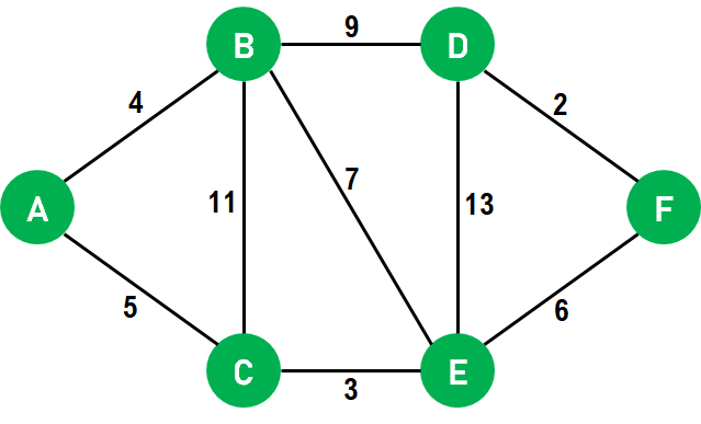
TEST CASE -3 :

A --1-- B --3-- C | / | 4 2 5 | / | D --6-- E --7-- F

INPUT:

Start Node: A End Node: F

OUTPUT:

Shortest Path: A -> B -> C -> F Shortest Distance: 9